Excel is one of the most versatile spreadsheet programs for PC users. It is a Microsoft spreadsheet program that calculates and stores statistical data. You can generate graphical reports using Excel. You can learn how to create a Report in Excel by reading this user-friendly guide.
Microsoft Excel is the earliest pioneer program for spreadsheets applications in the early 90s. Excel was originally a desktop application for professionals like accountants, mathematicians, and scientists. You can access Excel if you have a computer, tablet, or smartphone.
The modern Excel spreadsheet program is compact and relatively easy to acquire over the internet. The latest Excel program has lots of features that you can check out. You can check the Report feature in Excel and figure out how to create a Report in Excel.
Design Charts for Report Generation in Excel
You can use the following procedure to generate your Excel Report with visual elements like charts and tables.
Step 1: Open an Excel worksheet and populate it with random data. Ensure the data is logical and relatable to get the best practical experience.
Step 2: Click on the Insert tab at the top of your excel worksheet. Locate the Charts groups on the Insert Ribbon section.

Step 3: Select and click on your preferred Chart to include in your Excel Report.
Step 4: Locate the Chart Design menu and click Select Data under the Data group section.

Step 5: Select the Excel Sheet with your randomly populated data. Narrow down the Cells containing relevant data and Select them. You can use the Click, Hold and Drag motion to select nearby Cells in a wide area.
You can use the Click + pressing the CTRL key to select individual Cells in a wide area. Ensure your selection area covers Headers to get a detailed report with relevant Labels.
Step 6: Your Sheet will refresh and update your changes when you select your preferred type of Chart. Your Header will represent the X and Y-Axis Labels on your Chart Report.

Step 7: You can repeat the above process to generate a different report using the data saved in your Excel workbook.
Step 8: You can use the Copy & Paste function to generate a new Chart automatically and replicate your selected data.

Design PivotTables for Report Generation in Excel
Step 1: Open a New Excel file and use the Copy & Paste function to duplicate the previous random raw data to your new Sheet.
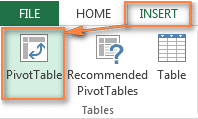
Step 2: Click on the Insert tab at the top of your Sheet. Locate the PivotTable option at the top left of your Ribbon screen section and click on it.
Step 3: Wait for the PivotTable Dialogue Window to launch, and click on the Table/Range field to select your preferred range of data.
Step 4: Select the Location field and click on the first cell where you want the PivotTable inserted. Click on the Ok button to complete the data selection and PivotTable location selection process.
Step 5: The new PivotTable generation process will commence on a New Sheet with your Selected Cell acting as the reference field.
Step 6: You can Import Data from your Excel file by Clicking and dragging your preferred fields to the New PivotTable field pane.
Step 7: Your new PivotTable will collate your data from multiple import sources by adding them to your new Sheet.
Step 8: You can refresh your data analysis by clicking on the Drop-Down Arrow next to your items in the Value Field Settings.
Step 9: Locate the Value Field Settings dialogue box to select your preferred Calculation Type by clicking on it.

Step 10: Your PivotTable data analysis updates will refresh and reflect whenever you adjust data importation from your source file.
Compile and generate PivotTables for the Dashboard
You can use the steps below to compile and generate multiple PivotTables on a Dashboard to represent your data.
Step 1: Select a master PivotTable that you would like to use as a master reference.
Step 2: Right-click on your preferred selection of data.
Step 3: Click on the Copy option before selecting a different cell on your Worksheet.
Step 4: Right-click on the selected cell before clicking the Paste option to duplicate your data.
Step 5: Repeat the procedure above to replicate other data selections on your Worksheet.
Step 6: Click on the Insert tab before clicking on the PivotTable Tools for each selected table.
Step 7: Click on the Analyze option to generate a graphical representation of your data.
Step 8: Ensure you insert your preferred name on the PivotTable Name box to label and identify your selected tables.

Print the Visual Excel Report after the Graph/PivotTable Generation Process
You can follow the following procedure to prepare and print the Visual Excel Reports that you have created.
Step 1: Go to your Graph/PivotTable Excel Report and click on the Insert tab above your Sheet.
 Step 2: Navigate to the top right of your Sheet and click on the Text option before clicking on the Header & Footer section.
Step 3: You can input the Title of your Report Page by typing your preferred page reference and formatting it using the larger text fonts on your Excel file.
Step 4: You can then hide the irrelevant sheets by Right-clicking on the Sheet tab and selecting the Hide option.
Step 5: To prepare your Report for printing, click on the File tab at the top left of your screen and click on the Print option. Go to the Printing Window Panel and change the Page Orientation to Landscape. Ensure the Scaling preference for your Page Setup is on Fit All Columns on One Page.
Step 6: Click on the Print Entire Workbook option to ensure your selected Report Sheets are added to your printing queue and printed whenever your Printer is active and available.

Step 7: You can return to the File tab and click on the Save As preference to save changes to our Excel file using your preferred file type.
Conclusion
You can import data from a Word document by clicking on the Data tab on Excel and then clicking on the Get External Data Wizard at the top left corner of your Worksheet.
You can save your Excel file using Excel 97-2003 Workbook file format to ensure the formatting styles in your file remain compatible even when using older versions of MS Office to open your Excel file.